Using Mean And Mean Absolute Deviation To Compare Data In I-Ready: A Complete Guide

Have you ever wondered how teachers and analysts can quickly tell if two groups of numbers are truly different, or if any observed difference is just random chance? This is the heart of using mean and mean absolute deviation to compare data in i-Ready and beyond. Whether you're a student navigating the i-Ready diagnostic, a teacher interpreting class results, or simply someone looking to make sense of data in everyday life, understanding these two fundamental statistical tools is your key to unlocking deeper insights. They transform raw, messy numbers into clear, comparable stories. This guide will walk you through everything you need to know, from basic definitions to advanced comparison techniques, using practical examples and direct applications to the i-Ready platform.

What Exactly Are Mean and Mean Absolute Deviation (MAD)?

Before we can compare, we must first understand our tools. The mean and mean absolute deviation (MAD) are the yin and yang of descriptive statistics—one tells you where the center is, and the other tells you how spread out the data is around that center.

Demystifying the Mean: The Average Anchor

The mean, often called the average, is the most common measure of central tendency. You calculate it by adding up all the data points and dividing by the number of points. It’s the balancing point of your data distribution. For example, if you have the test scores 85, 90, 78, and 92, the mean is (85+90+78+92)/4 = 86.25. This single number gives you a quick snapshot of the overall performance.

• Why it matters: The mean is sensitive to every value in the set. A single extremely high or low score (an outlier) can pull the mean up or down, which can be both a strength (it uses all data) and a weakness (it can be skewed).
• In i-Ready: Your overall diagnostic score is essentially a weighted mean across all the domains and standards you were tested on. It’s the primary "center" number you see.

Introducing MAD: The Spread Detective

While the mean tells you the center, the mean absolute deviation tells you about the variability or spread. Mean refers to the average of data points whereas mean absolute deviation measures how spread out these numbers are. It answers the question: "On average, how far is each data point from the mean?"

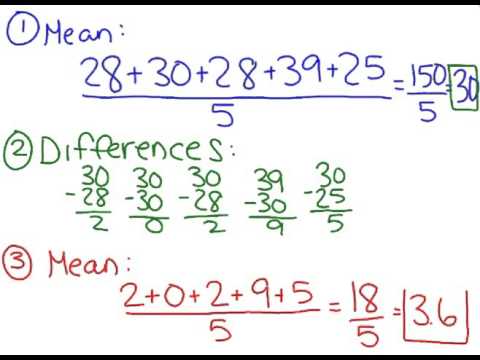
To calculate MAD:

1. Find the mean of your data set.
2. Calculate the absolute difference (positive distance) between each data point and the mean.
3. Find the mean of those absolute differences.

For our scores (85, 90, 78, 92) with a mean of 86.25:

• Differences: |85-86.25| = 1.25, |90-86.25| = 3.75, |78-86.25| = 8.25, |92-86.25| = 5.75
• MAD = (1.25 + 3.75 + 8.25 + 5.75) / 4 = 18/4 = 4.5

This means, on average, each score is 4.5 points away from the class average of 86.25. A small MAD indicates data points are clustered tightly around the mean (low variability). A large MAD means the data points are spread out (high variability).

• Why it matters: Two classes can have the same mean score but wildly different MADs. Class A with scores 85, 86, 87, 86 has a mean of 86 and a tiny MAD (~0.7), showing consistent mastery. Class B with scores 70, 90, 80, 100 has the same mean of 85 but a MAD of 10, showing huge performance swings. The mean alone hides this crucial story.

The Foundation: Levels of Measurement and Why They Matter

You cannot meaningfully calculate a mean or MAD for just any type of data. Further, data are classified into four levels of measurement, each allowing specific statistical operations. Using the wrong measure on the wrong data type leads to nonsense.

Level of Measurement	Description	Examples	Can Calculate Mean?	Can Calculate MAD?
Nominal	Categories with no order.	Eye color, animal type, brand names.	❌ No (averaging categories is meaningless)	❌ No
Ordinal	Categories with a ranked order, but no consistent interval.	Letter grades (A, B, C), satisfaction ratings (Very Satisfied to Very Dissatisfied).	⚠️ Controversial. The "average" of A and C isn't a real grade.	❌ No (intervals aren't equal)
Interval	Ordered data with consistent intervals, but no true zero.	Temperature in Celsius/Fahrenheit, IQ scores.	✅ Yes	✅ Yes
Ratio	Like interval, but with a meaningful, non-arbitrary zero.	Height, weight, age, test scores (0 = no correct answers).	✅ Yes	✅ Yes

Key Takeaway: The mean and MAD are interval/ratio level operations. The i-Ready scores you work with (scaled scores, diagnostic points) are carefully designed to be at least interval data, making these calculations valid and meaningful. You would never calculate the mean of student names or lunch choices.

The i-Ready Context: How This Applies to Students and Teachers

In grade 7, students continue their work with data display and analysis. This isn't new; it's a deepening of prior knowledge. In previous grades, they have described the shape of a data set and calculated mean, median, mode, and range. They have worked with dot plots and box plots. Now, in Grade 7 (aligned with standards like 7.SP.B.3 and 7.SP.B.4), the focus shifts to measures of variability like MAD and using them to informally assess the degree of visual overlap of two numerical data distributions.

This is precisely using mean and mean absolute deviation to compare data in i-Ready. The i-Ready Diagnostic provides individual student scores and class/group means and MADs (often in the "Data" or "Reports" sections for teachers). A student or teacher can look at two different standards, two different classes, or two different time periods and ask:

• Is the difference in average scores (means) large enough to be important?
• Is one group's performance more consistent than the other's (comparing MADs)?
• How much do the distributions overlap when visualized?

They learn measures of variability and use them to compare data sets. They assess the degree of visual overlap of two numerical data distributions. This skill is critical for moving beyond "Class A's average is higher" to "Class A's average is higher and their scores are much more consistent, indicating tighter instruction."

Step-by-Step: Comparing Two Data Distributions

Now, let's get practical. Let's learn how to describe and compare data distributions using the mean and the mean absolute deviation (MAD). The process is systematic.

Step 1: Calculate/Identify the Means.
Find the average score for each group (e.g., Class A vs. Class B on the Geometry domain).

Step 2: Calculate/Identify the MADs.
Find the average spread for each group. A smaller MAD means less variability.

Step 3: Compare the Means.
How large is the difference? Is it larger than the typical spread (MAD)? A good rule of thumb: if the difference in means is larger than the average of the two MADs, the distributions are likely to be "visually separate" with little overlap. If the difference is smaller than the MADs, the distributions will show significant overlap.

Step 4: Compare the MADs.
Is one group's performance much more consistent? A group with a lower MAD has more uniform scores, which might suggest effective, standardized teaching. A high MAD suggests some students are excelling while others are struggling, possibly indicating a need for differentiation.

Step 5: Synthesize a Conclusion.
Combine your findings. Example: "The mean score for Group 1 (78.5) is 5 points higher than Group 2 (73.5). However, Group 1's MAD (3.2) is nearly identical to Group 2's MAD (3.1). This suggests Group 1 consistently outperforms Group 2 across the board, not just at the extremes."

Practical Example: The Animal Clinic Scenario

Let's bring this to life with the example from the key sentences. There is a large difference in the mean number of stray cats rescued by a new leash on life animal clinic each week and the mean number of stray cats taken in by no ruff stuff animal hospital each week. The mean number of cats treated each day at no ruff stuff animal hospital is lower than the mean number of cats treated each day at a new leash on life animal clinic.

Imagine we have weekly data for 10 weeks:

• New Leash on Life (NLOL): 12, 15, 14, 16, 13, 15, 17, 14, 16, 15
• No Ruff Stuff (NRS): 8, 9, 7, 10, 8, 9, 11, 8, 9, 8

Calculations:

• NLOL Mean: (12+15+14+16+13+15+17+14+16+15)/10 = 147/10 = 14.7 cats/week
• NRS Mean: (8+9+7+10+8+9+11+8+9+8)/10 = 87/10 = 8.7 cats/week
• Difference: 14.7 - 8.7 = 6.0 cats/week. The difference between the mean... is about 6.
• NLOL MAD: Calculate absolute deviations from 14.7: (2.7, 0.3, 0.7, 1.3, 1.7, 0.3, 2.3, 0.7, 1.3, 0.3). Mean of these = 11.0/10 = 1.1.
• NRS MAD: Deviations from 8.7: (0.7, 0.3, 1.7, 1.3, 0.7, 0.3, 2.3, 0.7, 0.3, 0.7). Mean = 9.0/10 = 0.9.

Analysis: There is a clear and substantial difference in the means (6 cats). The MADs are very small and similar (1.1 vs. 0.9), meaning both clinics have very consistent weekly intake numbers. The large difference in means is not due to one clinic being erratic; it's a consistent, significant disparity in their average workload. NLOL consistently rescues about 6 more stray cats per week than NRS.

Advanced Comparison: The Basketball Team Height Example

Now, let's look at a case where the means are different but the spreads are similar, as hinted in the key sentences. The difference between the mean heights of the teams is about 6 (77.2 - 71.5). The mad for the two distributions are about the same (between 2.3 and 2.4).

Imagine two basketball teams:

• Women's Team Heights (in): 75, 78, 76, 80, 77, 74, 79, 76, 78, 77
• Men's Team Heights (in): 70, 72, 71, 73, 69, 74, 71, 72, 70, 71

Calculations (Rounded):

• Women's Mean: ~77.2 in. You can use the same procedure to compute the women’s team’s mad, which in this case would equal 2.3 (rounded to the nearest tenth).
• Men's Mean: ~71.5 in. Difference = ~5.7 in (about 6).
• Women's MAD: ~2.3 in.
• Men's MAD: ~2.4 in.

Analysis: The men's team is, on average, about 6 inches shorter. The mad for the two distributions are about the same. This tells us that the spread of heights is nearly identical within each team. The height distributions are essentially the same shape, just shifted (offset) by about 6 inches. There would be significant overlap in the heights—some of the tallest women might be taller than some of the shortest men. The difference in means is meaningful, but the similar MADs tell us the variability is consistent across both groups.

Common Pitfalls and How to Avoid Them

When using mean and mean absolute deviation to compare data in i-Ready or any analysis, watch out for these traps:

1. Ignoring the MAD: This is the #1 mistake. Reporting only the mean is like reporting the average temperature of a city without mentioning if it's stable or has brutal swings. What can you tell about the mean of each distribution? You can tell the center, but you know nothing about reliability or consistency without the MAD.
2. Comparing Means with Huge MADs: If Group A has a mean of 80 (MAD: 15) and Group B has a mean of 85 (MAD: 14), the 5-point difference is smaller than the typical spread. The distributions likely overlap greatly. Claiming Group B is "better" based on mean alone is misleading.
3. Using Mean/MAD on Ordinal Data: Do not calculate these for letter grades or rank orders. The math doesn't represent real distances.
4. Being Fooled by Outliers: The mean is sensitive to extreme values. If comparing two small classes, one student's exceptionally high or low score can distort the mean. In such cases, the median might be a better center measure, but remember, you can't then calculate a "median absolute deviation" in the same simple way for comparison. Check the raw data or a box plot.
5. Overlooking Sample Size: A mean difference based on 5 data points is far less reliable than one based on 500. i-Ready reports often include sample size (n) for a reason.

Actionable Tips for i-Ready Users

• For Students: When you see your i-Ready report, don't just look at your overall score. Ask: "Is my mean score in this domain above grade level? What's my MAD (sometimes shown as 'average distance from mean' or variability)? A low MAD means your performance is steady. A high MAD means you have some strong and some weak standards—talk to your teacher about that pattern."
• For Teachers: In your i-Ready class reports, use the mean to compare overall class performance across standards or time. Use the MAD (or the related "standard deviation" if available) to gauge class consistency. A class with a high mean but also a high MAD has a wide spread of understanding—you'll need small-group instruction. A class with a moderate mean and low MAD is fairly uniform. Compare the difference in means between two groups to their average MADs to judge if the gap is substantial.
• For Everyone: Always visualize if possible. Sketch a simple dot plot or box plot for each group. The mean is the balance point; the MAD gives you a sense of the "width" of the cloud of dots. Does one cloud sit clearly to the right of the other? Or do they sit on top of each other?

Conclusion: Beyond the Numbers to True Understanding

Mastering using mean and mean absolute deviation to compare data in i-Ready transforms you from a passive consumer of statistics into an active interpreter of information. The mean gives you the landmark—the central tendency. The mean absolute deviation gives you the terrain—the consistency and spread around that landmark. Together, they answer the critical questions: Where is the center? How reliable is that center? How do two groups truly differ?

Remember the animal clinic: the large difference in means with tiny, similar MADs told a story of consistently different workloads. Remember the basketball teams: the similar MADs told us the height spread was identical, even if the average height differed. This nuanced understanding is what separates surface-level observation from meaningful analysis.

So, the next time you encounter a set of numbers—in an i-Ready report, a business dashboard, or a news article—pause. Find the mean. Then, find the MAD. Ask how they compare. This simple, powerful two-step process will reveal the real story hidden in the data, allowing for smarter decisions, targeted interventions, and a profound appreciation for the beautiful logic of statistics. The numbers are talking; now you know how to listen.