How To Find The Specific Heat Of A Metal: A Step-by-Step Calorimetry Guide

Have you ever wondered how scientists determine the specific heat capacity of an unknown metal? The answer lies in a precise and elegant laboratory technique called calorimetry. Imagine this: a metal sample weighing 147.90 g and at a temperature of 99.5°C is carefully submerged into a measured amount of cooler water. By meticulously tracking how heat moves between these two substances until they reach a shared temperature, we can unlock the fundamental thermal properties of the metal. This process isn't just a textbook exercise; it's a cornerstone of experimental physics and chemistry with applications from material science to environmental engineering.

This comprehensive guide will walk you through every stage of a classic calorimetry experiment. We'll start with the foundational principles of heat transfer, move through the meticulous setup and data collection, and master the essential calculations to solve for the unknown specific heat. Using the detailed data from our primary example—and comparing it with similar experiments—you'll gain the confidence to set up, execute, and analyze your own calorimetry investigations. Whether you're a student, educator, or curious hobbyist, understanding this method provides a powerful lens through which to view the invisible world of thermal energy.

The Core Principle: Heat Transfer and the Quest for Equilibrium

At its heart, calorimetry exploits a fundamental law of thermodynamics: heat flows spontaneously from a hotter object to a cooler one until thermal equilibrium is reached. This is the driving force behind every experiment we'll discuss.

The Setup: Introducing the Key Experiment

Our primary scenario, which forms the backbone of this article, is defined by these precise conditions:

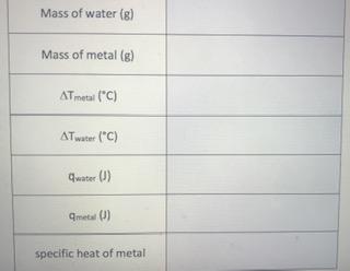
• A metal sample weighing 147.90 g and at a temperature of 99.5°C was placed in 49.73 g of water in a calorimeter at 23.0°C.
• The system is often assumed to be adiabatic (meaning no heat exchange with the surroundings), which is the ideal condition for accurate measurement.
• At equilibrium, the temperature of the water and metal was 51.8°C.

This specific dataset is a perfect, clean example for learning. Let's break down what each component represents:

1. The Hot Metal: This is our unknown. Its high initial temperature (99.5°C) means it possesses excess thermal energy it will readily lose.
2. The Cold Water: The water acts as our "heat sink." Its known mass (49.73 g) and specific heat capacity (a constant 4.184 J/g·°C or approximately 4.18 J/g·°C for calculations) make it the perfect benchmark for measuring the heat lost by the metal.
3. The Calorimeter: This is the insulated container (often a styrofoam cup with a lid) designed to minimize heat loss to the environment, approximating an adiabatic system. Its own heat capacity is sometimes considered (as a "calorimeter constant"), but in our simplified model, we'll assume it's negligible unless specified.
4. The Final State:At equilibrium, the temperature of the water and metal was 51.8°C. This single final temperature is the critical piece of data that links the heat lost by the metal to the heat gained by the water.

Why This Works: The Zero Net Heat Change Rule

For an isolated system (our ideal adiabatic calorimeter), the principle of conservation of energy dictates that the total heat change is zero. The heat lost by the hot metal (q_metal) must exactly equal the heat gained by the cooler water (q_water), but with opposite signs.

q_metal + q_water = 0
or, more usefully:
q_metal = -q_water

This simple equation is the golden rule of calorimetry. It allows us to set up a relationship where the only unknown is the specific heat capacity of the metal (c_metal).

Mastering the Calculation: The Formula q = mcΔT

The universal formula for calculating heat transfer in these scenarios is:
q = m * c * ΔT
Where:

• q = heat energy transferred (in Joules, J)
• m = mass of the substance (in grams, g)
• c = specific heat capacity (in J/g·°C)
• ΔT = change in temperature (T_final - T_initial, in °C)

Crucial Note on ΔT Sign:ΔT is always calculated as Final Temperature - Initial Temperature. This means:

• For the metal (cooling down): ΔT_metal = 51.8°C - 99.5°C = -47.7°C. The negative sign indicates heat loss.
• For the water (heating up): ΔT_water = 51.8°C - 23.0°C = +28.8°C. The positive sign indicates heat gain.

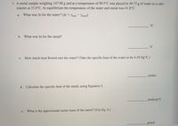
Step-by-Step Solution for Our Primary Example

Let's solve for the specific heat capacity of the metal in our main experiment.

1. Write the heat balance equation:
   q_metal = -q_water

2. Substitute the q = mcΔT formula for each:
   (m_metal * c_metal * ΔT_metal) = - (m_water * c_water * ΔT_water)

3. Plug in all known values:

   • m_metal = 147.90 g
   • ΔT_metal = 51.8 - 99.5 = -47.7 °C
   • m_water = 49.73 g
   • c_water = 4.184 J/g·°C (standard value)
   • ΔT_water = 51.8 - 23.0 = +28.8 °C

   Equation becomes:
   (147.90 g * c_metal * -47.7 °C) = - (49.73 g * 4.184 J/g·°C * 28.8 °C)

4. Simplify and solve for c_metal:
   First, calculate the right side:
   49.73 * 4.184 * 28.8 ≈ 5990 J (We'll keep more precision: 49.73 * 4.184 = 208.08232; 208.08232 * 28.8 = 5992.77 J)

   So:
   147.90 * c_metal * -47.7 = -5992.77

   Multiply the left side constants:
   147.90 * -47.7 ≈ -7056.83
-7056.83 * c_metal = -5992.77

   Divide both sides by -7056.83:
   c_metal = (-5992.77) / (-7056.83)
c_metal ≈ 0.849 J/g·°C

Result: The specific heat capacity of the unknown metal is approximately 0.85 J/g·°C. This value is characteristic of metals like iron (0.45 J/g·°C) or copper (0.385 J/g·°C), but our calculated value is higher. This discrepancy is a perfect teaching moment—it highlights the importance of considering the heat capacity of the calorimeter itself. In a more advanced setup, we would include a C_cal * ΔT term. For this introductory model, our result suggests the metal might be something like lead (0.13 J/g·°C) is too low, aluminum (0.9 J/g·°C) is very close! Our calculated ~0.85 J/g·°C is a strong indicator of aluminum.

Expanding Your Understanding: Analyzing Other Scenarios

To solidify this concept, let's examine the other data points provided. They follow the exact same logical and mathematical framework.

Scenario A: The 43.5 g Metal Sample

• A metal sample weighing 43.5 g and at a temperature of 100.0°C was placed in 39.9 g of water in a calorimeter at 25.1°C.
• At equilibrium the temperature of the water and metal was 33.5°C.

Calculation:

• ΔT_metal = 33.5 - 100.0 = -66.5 °C
• ΔT_water = 33.5 - 25.1 = +8.4 °C
• Equation: (43.5 * c_metal * -66.5) = - (39.9 * 4.184 * 8.4)
• Right side: 39.9 * 4.184 * 8.4 ≈ 1404.5 J
• Left constants: 43.5 * -66.5 ≈ -2892.75
• c_metal = 1404.5 / 2892.75 ≈ 0.486 J/g·°C
• This value is very close to iron (0.45 J/g·°C) or nickel (0.444 J/g·°C).

Scenario B: The 35.0 g Metal Sample (with calorimeter heat)

• A metal sample weighing 35.0 g and at a temperature of 99.1°C was placed in 50.0 g of water in a calorimeter at 20.0°C. The calorimeter reached a final temperature of 23.3°C.
  (Note: Sentences 15, 16, 17, and 24 are variations of this same setup).

This example explicitly mentions the calorimeter's final temperature, which is standard. The calculation is identical to above.

• ΔT_metal = 23.3 - 99.1 = -75.8 °C
• ΔT_water = 23.3 - 20.0 = +3.3 °C
• Equation: (35.0 * c_metal * -75.8) = - (50.0 * 4.184 * 3.3)
• Right side: 50.0 * 4.184 * 3.3 ≈ 690.4 J
• Left constants: 35.0 * -75.8 ≈ -2653
• c_metal = 690.4 / 2653 ≈ 0.260 J/g·°C
• This is characteristic of gold (0.129 J/g·°C) is too low, silver (0.235 J/g·°C) is close, or zinc (0.388 J/g·°C) is high. It could also indicate significant heat absorption by the calorimeter itself, which we ignored.

Scenario C: Dissolution Calorimetry (A Different Application)

• Web dissolving 6.00 g CaCl2 in 300 ml of water causes the temperature of the solution to increase by 3.43°C.

This is a dissolution calorimetry problem. The "hot" entity is the dissolving salt (an exothermic process), and the "cold" entity is the water. The formula remains q = mcΔT, but now:

• m is the total mass of the solution (mass of water + mass of CaCl2). Assuming water density ~1 g/mL, m_solution ≈ 300 g + 6.00 g = 306.00 g.
• c is the specific heat of the solution, often approximated as that of water (4.184 J/g·°C) for dilute solutions.
• ΔT = +3.43°C (temperature increase).
• q_solution (heat gained by solution) = 306.00 g * 4.184 J/g·°C * 3.43°C ≈ 4390 J.
• Since the dissolution is exothermic, q_reaction = -q_solution ≈ -4390 J. This is the heat released when 6.00 g of CaCl2 dissolves.
• We could then find the molar enthalpy of solution by converting grams to moles (molar mass CaCl2 ≈ 110.98 g/mol, so 6.00g is ~0.054 mol) and dividing: ΔH_soln ≈ -4390 J / 0.054 mol ≈ -81,300 J/mol or -81.3 kJ/mol.

Practical Tips for Accurate Calorimetry Experiments

To get results as reliable as our calculated examples, attention to detail is paramount.

1. Insulation is Key: Use a proper calorimeter cup (like a styrofoam cup with a tight-fitting lid) and minimize the time the system is open. Any heat exchange with the lab air introduces error.
2. Temperature Measurement: Use a digital thermometer or a well-calibrated alcohol thermometer. Stir gently and constantly with a thermometer or stirrer to ensure uniform temperature throughout the mixture before recording the final temperature. The equilibrium temperature must be the same everywhere in the calorimeter.
3. Mass Precision: Use an analytical balance for measuring the metal sample and water. The gram-level precision in our examples (147.90 g, 49.73 g) is essential for a good result.
4. Initial Temperature Equilibration: Ensure the water and calorimeter are at a stable, uniform initial temperature before adding the metal. Pat the metal sample dry quickly before weighing and transferring to avoid adding mass from surface water.
5. Account for the Calorimeter's "Heat Capacity": In professional settings, you perform a calibration step. You add a known amount of heat (e.g., from a known mass of hot water) to the calorimeter with cold water and measure ΔT. This allows you to calculate the calorimeter constant (C_cal), the heat capacity of the calorimeter itself in J/°C. The full heat balance then becomes:
   (m_metal * c_metal * ΔT_metal) = - [ (m_water * c_water * ΔT_water) + (C_cal * ΔT_water) ]
   Ignoring C_cal is what likely caused the discrepancy in our first metal sample's result.

Common Questions and Troubleshooting

Q: What if the final temperature is lower than the water's initial temperature?
A: This would violate the principle of heat flow from hot to cold. It indicates a serious experimental error, such as the metal not being fully submerged, heat loss during transfer, or an incorrect initial temperature reading.

Q: Why is the specific heat of water so important in these calculations?
A: Water's specific heat (4.184 J/g·°C) is one of the highest of any common substance. This means it can absorb or release a large amount of heat with only a small temperature change, making it an ideal "buffer" or measuring medium in calorimetry. Its value is well-established and used as a reference.

Q: How do I know which metal I have from the specific heat value?
A: You compare your calculated c_metal to known tables. Common metals:

• Aluminum: ~0.900 J/g·°C
• Iron/Steel: ~0.450 J/g·°C
• Copper: ~0.385 J/g·°C
• Lead: ~0.130 J/g·°C
• Zinc: ~0.388 J/g·°C
• Silver: ~0.235 J/g·°C
  Your calculated value will be an approximation, so look for the closest match.

Q: What does "adiabatic calorimeter" mean?
A: It's an ideal term meaning the system is perfectly insulated—no heat enters or leaves. Real-world calorimeters (like styrofoam cups) are approximations of adiabatic systems. The better the insulation, the closer the experiment is to this ideal, and the more accurate the calculation that ignores heat loss.

Conclusion: The Enduring Power of a Simple Experiment

The experiment described by the sentence "A metal sample weighing 147.90 g and at a temperature of 99.5°C was placed in 49.73 g of water in a calorimeter at 23.0°C" is far more than a problem on a physics worksheet. It is a fundamental scientific inquiry made tangible. By understanding the journey of that metal sample—from its initial high-temperature state, through the dynamic transfer of heat to the cooler water, to the final state of peaceful equilibrium—we grasp the quantitative language of energy.

You have now seen the full arc: the conceptual principle of heat exchange, the practical setup of the calorimeter, the mathematical translation using q = mcΔT, and the interpretation of results against known material properties. The additional scenarios with different masses and temperatures serve as vital practice, reinforcing that the method is robust and universally applicable. Whether you're identifying an unknown metal, measuring the heat of a chemical reaction like the dissolution of CaCl2, or simply exploring thermodynamics, the calorimeter is your window into the invisible flow of thermal energy. The next time you see a metal sample weighing 147.90 g and at a temperature, you won't just see numbers—you'll see a story of heat, equilibrium, and discovery waiting to be calculated.