Demystifying Consumer Surplus: How To Read The Hidden Benefits On A Market Graph
Have you ever bought something and felt you got a fantastic deal, a true bargain that left you happier than you expected? That satisfying feeling isn't just a win in your wallet—it's a measurable economic concept called consumer surplus. But how do economists and analysts actually see this "hidden benefit" for an entire group of buyers? The answer lies in a simple yet powerful visual tool: the market graph. By learning to interpret these charts, you unlock a deeper understanding of market efficiency, welfare, and the real impact of policies like taxes. This comprehensive guide will walk you through everything you need to know about identifying and calculating consumer surplus for a group of consumers on a graph, transforming you from a casual observer into an informed interpreter of market dynamics.
What Exactly is Consumer Surplus? The Core Economic Benefit
At its heart, consumer surplus shows the extra benefit consumers get when they pay less than what they are willing to pay. It’s the monetary value of the gap between a buyer's maximum willingness to pay for a good or service and the actual price they pay in the market. This surplus represents the satisfaction or utility a consumer derives from participating in market transactions, essentially quantifying "getting more value than you paid for."
Imagine you’re in the market for a new smartphone. You’ve decided you’re willing to pay up to $1,200 for a specific model because of its features. If you find it on sale for $900, your consumer surplus is $300. That $300 is your economic gain, the extra happiness or utility you secured because the market price was below your personal valuation. When we aggregate this across all consumers in a market—from those willing to pay very high amounts to those barely willing to buy at the going price—we get the total consumer surplus for that group. This total is a critical component of total market welfare, which is the sum of all benefits to buyers and sellers.
The Perfect Market Graph: Visualizing Consumer Surplus
To see this aggregate benefit, we turn to the classic supply and demand graph. This chart graphically illustrates consumer surplus in a market without any monopolies, binding price controls, or any other inefficiencies—what economists call a perfectly competitive market. In this ideal scenario, the market reaches a state of Pareto optimality, where the price is set at the equilibrium point that maximizes total surplus without making anyone worse off.
On this graph, the demand curve slopes downward, reflecting the law of demand: as price decreases, the quantity demanded increases. Each point on the demand curve represents a specific consumer’s (or group of consumers') willingness to pay for an additional unit. The supply curve slopes upward, showing how much sellers are willing to provide at different prices. Their intersection determines the equilibrium price and equilibrium quantity.
The somewhat triangular area labeled by a letter (like 'f' in many textbook examples) in the graph shows the area of consumer surplus. This triangle is formed by three boundaries: the horizontal line at the equilibrium price, the vertical axis (price), and the demand curve itself. The fact that this area exists and is triangular visually demonstrates that the equilibrium price in the market was less than what many of the consumers were willing to pay. The height of the triangle at any quantity represents the difference between willingness to pay and the actual price for those marginal buyers.
Step-by-Step: How to Find Consumer Surplus on a Graph
So, how to find consumer surplus on a graph? It’s a straightforward geometric calculation once you identify the correct area. To find the consumer surplus on a graph, we calculate the area between the equilibrium price line and the demand curve, from zero up to the equilibrium quantity.
Here is the practical, actionable method:
- Locate the Equilibrium: Find the point where the supply and demand curves intersect. Note the equilibrium price (P*) and equilibrium quantity (Q*).
- Identify the Boundaries: The base of the consumer surplus triangle is the equilibrium quantity (Q*) on the horizontal axis. The left side is the vertical axis (price). The hypotenuse is the segment of the demand curve from the origin up to the equilibrium point.
- Calculate the Area: The formula for the area of a triangle is ½ × Base × Height.
- Base = Equilibrium Quantity (Q*)
- Height = The difference between the price intercept of the demand curve (where it meets the price axis, representing the highest willingness to pay) and the equilibrium price (P*).
- Consumer Surplus = ½ × (Q*) × (Max Willingness to Pay - P*)
Important Note: This simple triangular calculation assumes a linear demand curve. For a curved demand function, you would use integral calculus to find the exact area, but the conceptual understanding remains the same: it's the area under the demand curve and above the price level.
Deeper Dive: Supply, Demand, and Surplus Components
To fully master the graph, you must understand the functions and curves it represents. Supply and demand are the foundational models. The demand function mathematically relates the quantity demanded to the price, holding other factors constant. Its graphical representation, the demand curve, is the map of consumer willingness to pay. The supply function relates the quantity supplied to the price, and the supply curve represents the sellers' marginal costs.
On the same graph, the area above the supply curve and below the equilibrium price is the producer surplus—the benefit sellers receive for selling at a price higher than their minimum acceptable price (marginal cost). Consumer surplus and producer surplus are the two pillars of market wellness. Studying their relationship reveals the efficiency of the market mechanism. When these two areas are maximized at the equilibrium, the market is said to be allocatively efficient.
The Real-World Twist: How Taxes Disrupt the Surplus
Perfect markets are a baseline. Real-world interventions, like taxes, create "deadweight loss" and shrink the total surplus. An indirect tax (VAT), for instance, weighs on the consumer but is formally paid by large entities like corporations. However, the economic burden is partially shifted towards the consumer through a higher market price. This tax does not cause a direct loss of surplus for the producer in the same way it erodes consumer utility; instead, it creates a wedge between what buyers pay and what sellers receive.
On a graph with a per-unit tax, the supply curve shifts upward by the amount of the tax. The new equilibrium features a higher price paid by buyers and a lower price received by sellers (after tax). The consumer surplus shrinks significantly. To analyze this, you would indicate each area on the graph with a letter and show in a table the consumer surplus and the producer surplus before and after the tax. You would also indicate the dead weight loss associated with this tax, which is the small triangular area representing the lost surplus from the mutually beneficial trades that no longer occur due to the tax-induced price distortion. The tax creates inefficiency, reducing the total pie of market welfare.
A Concrete Example: Satellite TV Service Market
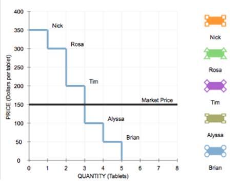
Let's apply this to a specific scenario. The graph shows the market demand for satellite TV service. Suppose the market price is $81. Which consumers receive consumer surplus in this market?
Looking at the demand curve, every consumer whose willingness to pay is greater than $81 receives a surplus. Those willing to pay exactly $81 have a surplus of zero—they are indifferent. Those willing to pay something less than $81 do not purchase the service at $81 and thus receive no surplus from this market transaction. The total consumer surplus is the area of the triangle above the $81 price line and below the demand curve, from zero to the quantity demanded at $81 (say, 16,000 subscribers per year). This visual instantly tells us that the 16,000th subscriber has a willingness to pay of exactly $81, while the first subscriber has a willingness to pay at the very top of the demand curve.
Beyond the Graph: Total Surplus and Market Wellbeing
The total surplus in a market is a measure of the total wellbeing of all participants in a market. It is the sum of consumer surplus and producer surplus. This total represents the maximum possible gains from trade in that market. When total surplus is maximized at the competitive equilibrium, resources are allocated to those who value them most highly (as shown by the demand curve) and produced by those who can do so at the lowest cost (as shown by the supply curve).
Policies that create deadweight loss, like taxes, price ceilings, or price floors, reduce this total surplus. The goal of economic policy is often to maximize this total while considering equity (how the surplus is distributed). Both consumer surplus and producer surplus determine market wellness by studying the relationship between the consumers and suppliers. A healthy, efficient market generates large, growing surpluses for both sides.
Practical Tools and Modern Applications
For those who want to compute these values without manual graphing, the consumer surplus calculator is a handy tool that helps you compute the difference between what consumers are willing to pay for a good or service versus its market price. You typically input the demand function or a set of willingness-to-pay data and the market price to get the total area.
Understanding consumer surplus also connects to the concept of marginal utility. The demand curve is derived from the utility consumers get from each additional unit. The height of the demand curve at any quantity is the marginal willingness to pay, which equals the marginal utility in dollar terms. The consumer surplus from the first unit is the difference between its high marginal utility and the low market price, highlighting how markets allow consumers to gain high utility at an average cost.
A Real-World Anomaly: The Discontinuation of the Penny
An unexpected real-world event that tangentially touches on concepts of exact pricing and consumer surplus is the discontinuation of the penny by the U.S. Mint. The Alert the division of consumer affairs has issued a “consumer and business advisory” regarding the discontinuation of the penny and the impact this is having on providing exact change for consumers paying for goods and services with cash.
While seemingly small, this change forces rounding of cash transactions to the nearest nickel. For individual purchases, the effect on consumer surplus is minuscule. However, aggregated across billions of transactions, it represents a systematic, tiny transfer of value. In some cases, rounding rules might slightly favor consumers; in others, businesses. It’s a practical example of how the granularity of price setting can subtly influence the distribution of economic surplus, even if it doesn't significantly alter the overall demand curve or total market surplus for most goods. It highlights that the "price" on the graph is often a simplified average, and real-world transaction mechanics can create small deviations.
Interpreting Real Data: City Averages and Expenditure Categories
When looking at official economic data, you might encounter reports like City average, by expenditure category. These breakdowns (e.g., for food, housing, transportation) allow for a more nuanced view of consumer surplus. Different categories have different demand elasticities. For necessities with inelastic demand (like medicine), the consumer surplus area might be smaller because willingness to pay doesn't drop sharply with quantity. For goods with elastic demand (like restaurant meals), the area can be larger. Analyzing these categories helps policymakers understand where consumer welfare is most sensitive to price changes.
Conclusion: The Lasting Value of Graphical Literacy
Understanding consumer surplus for a group of consumers on a graph is far more than an academic exercise. It is a fundamental literacy for anyone interested in economics, business, or public policy. The simple triangular area on a supply and demand graph encapsulates the essence of market benefit—the idea that voluntary exchange creates value for both parties. By learning to find consumer surplus on a graph, you gain the ability to visually assess market efficiency, predict the impact of taxes and subsidies, and critically evaluate claims about pricing and welfare.
From the theoretical Pareto optimal equilibrium to the messy reality of indirect taxes and even the rounding effects of a discontinued penny, the principles of consumer surplus provide a consistent framework. It reminds us that the price tag is only part of the story; the true value lies in the difference between what we pay and what we truly believe a product is worth. The next time you see a supply and demand chart, look for that triangular area—it’s telling you the story of collective consumer gain, a silent measure of economic well-being generated by the market itself.