How Many Solutions Are There To This Nonlinear System? Unpacking The Apex Of Uncertainty

Feb 21, 2026 • minute read

Contents

Introduction: The Perplexing Question at the Apex of Algebra

So, you’re staring at a system of equations. It’s not the neat, tidy kind with straight lines. Instead, you’ve got curves—a parabola, a circle, maybe a cubic function. You pose the crucial question: “How many solutions are there to this nonlinear system?” You’re hoping for a clear, predictable answer, a formula or a theorem that hands you a number. But here’s the fascinating, frustrating, and ultimately liberating truth at the apex of this mathematical inquiry: unlike the predictable world of linear systems, there is no grand solvability theorem for nonlinear systems. There is no single, universal rule that says, “If you have equations of this type, you will always have n solutions.” The answer could be zero, one, two, three, or even an infinite number. This very uncertainty is what makes nonlinear systems a captivating and essential frontier in mathematics and its real-world applications.

This article is your comprehensive guide through that frontier. We will move beyond the simple question to understand why the answer is so variable, how we find whatever solutions do exist, and why this messy, unpredictable mathematics is the language of our universe. Whether you're a student grappling with homework, an educator seeking clarity, or a professional in a STEM field, understanding the behavior of nonlinear systems is crucial. Most natural and engineered systems are inherently nonlinear, and their solutions tell us everything from how populations grow to how bridges sway. Prepare to have your assumptions challenged and your problem-solving toolkit expanded.

What Exactly Is a Nonlinear System of Equations?

Before we can count solutions, we must define our territory. A system of equations where at least one equation is not linear is called a nonlinear system. A linear equation, as a refresher, is one where the highest power of any variable is 1 (e.g., y = 2x + 3). Its graph is always a straight line. A nonlinear equation, therefore, is any equation that is not of the first degree. This means it has a degree of two or more.

Key Examples of Nonlinear Equations:

Quadratic:y = x² - 4 (Parabola)
Circular:x² + y² = 25 (Circle)
Cubic:y = x³ - x
Exponential:y = e^x
Rational:y = 1/x

When these are paired in a system—say, with another quadratic, a linear equation, or another curve—we enter the realm of nonlinear systems. Just as with systems of linear equations, a solution of a nonlinear system is an ordered pair (or triple, etc.) that makes both equations true. It is the point (or points) of intersection on a graph. This geometric interpretation is our most powerful intuitive tool.

The Heart of the Mystery: Why There’s No Simple Answer

This is the core concept derived from our key sentences. Unlike linear systems, where two equations in two variables almost always yield one unique solution (unless they are parallel or coincident), nonlinear systems break all the rules.Except in special cases (for example, polynomials), we cannot tell a priori how many unique solutions exist for a nonlinear equation. There is no equivalent of the determinant test for linear systems.

So, when you’re faced with a nonlinear system, and you ask, “how many solutions are there?”, prepare yourself for an answer that could be 0, 1, 2, 3, or even a whole bunch more! This isn't a failure of mathematics; it's a reflection of the incredible diversity of shapes that curves can take. Two curves can:

Miss each other completely (0 solutions)
Touch at a single tangent point (1 solution)
Cross at two distinct points (2 solutions)
Intersect at three, four, or more points (imagine a cubic curve crossing a parabola)
Coincide partially or entirely, leading to infinitely many solutions (e.g., x² + y² = 1 and 2x² + 2y² = 2 describe the same circle).

The number of solutions to a nonlinear system depends on how the graphs of the equations intersect. They can have no solutions, one solution, or multiple solutions based on their geometric relationship. This variability is the apex of the challenge and the starting point of the investigation.

Visualizing the Possibilities: A Geometric Journey

Let’s ground this abstract variability in concrete, visual examples. The most common introductory case is the intersection of a parabola and a line.

Case 1: The Line and the Parabola

Consider the system:

y = x² - 4x + 3 (A parabola opening upwards)
y = 2x - 2 (A line)

Graphically, three scenarios are possible:

Two Solutions: The line cuts through the parabola at two distinct points.
One Solution: The line is tangent to the parabola, touching it at exactly one vertex point.
Zero Solutions: The line is entirely above or below the parabola's vertex, never crossing it.

This pattern extends to all curve combinations. A circle and a line can intersect 0, 1, or 2 times. Two ellipses can intersect up to 4 times. The theoretical maximum number of intersections for two polynomial equations of degrees m and n is mn* (Bézout's Theorem), but this maximum is not always achieved. It can have 0 (no intersection), 1 (tangent point), 2 or more (multiple intersections), or infinitely many if the equations describe the same curve.

The Algebraic Arsenal: Solving Nonlinear Systems

While graphs give us intuition, we need algebraic methods to find precise solutions. The two primary methods are direct adaptations from linear systems, but with critical differences.

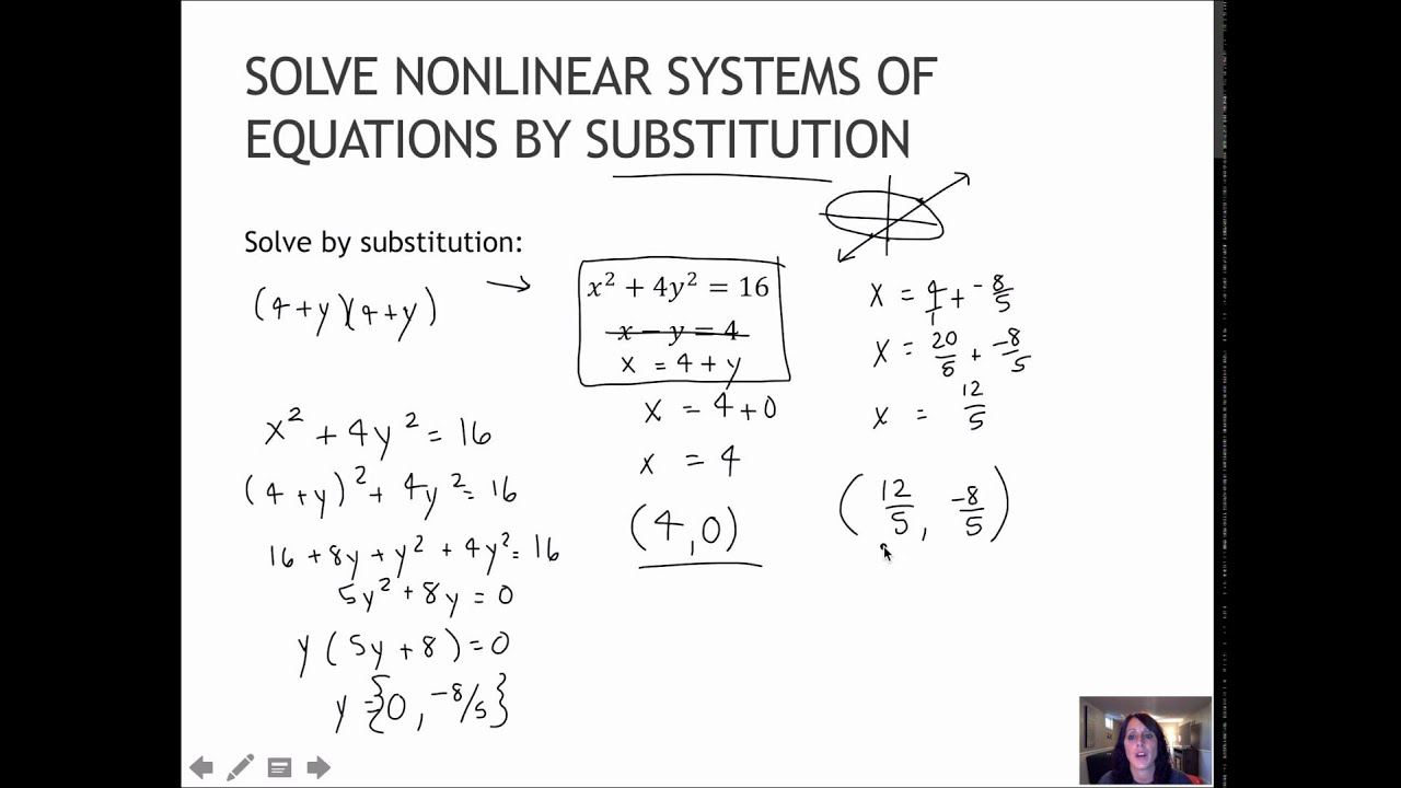
1. The Substitution Method: The Most Reliable Workhorse

We solve one equation for one variable and then substitute the result into the second equation to solve for another variable, and so on. This is often the preferred first strategy, especially when one equation is already solved for a variable (like y = ...) or can be easily manipulated.

Step-by-Step Example:
Solve:

x² + y = 5
x - y = -1

Step 1: Solve the simpler (often linear) equation for one variable. From equation 2: y = x + 1.
Step 2: Substitute this expression into the other equation. x² + (x + 1) = 5.
Step 3: Solve the resulting single-variable equation. x² + x - 4 = 0. This is a quadratic! Use the quadratic formula: x = [-1 ± √(1 + 16)] / 2 = [-1 ± √17]/2.
Step 4: Substitute eachx value back into y = x + 1 to find the corresponding y values.
Result: Two real solutions: ( (-1+√17)/2 , (1+√17)/2 ) and ( (-1-√17)/2 , (1-√17)/2 ).

A Pro Tip from the Key Sentences:If you are asked to solve a system of equations in which there is no linear equation to start with you can sometimes begin by isolating and substituting a variable that is squared in both equations. For example, in x² + y² = 25 and x² - y = 5, solving the second for x² (x² = y + 5) and substituting into the first is brilliant: (y+5) + y² = 25 → y² + y - 20 = 0.

2. The Elimination Method: Less Common, But Powerful

We learn how to solve nonlinear systems of equations algebraically by using the substitution method and the elimination method in order to find all solutions, both real and complex. Elimination works by adding or subtracting equations to cancel a variable. It’s most effective when equations have similar terms. For instance, with x² + y² = 10 and x² - y² = 2, simply add them to eliminate y², yielding 2x² = 12 → x² = 6.

Beyond Algebra: The Critical Role of Graphing

The solution to a nonlinear system of inequalities is the region of the graph where the shaded regions of the graph of each inequality overlap, or where the regions intersect, called the feasible region. While our focus is on equations, this graphical principle is paramount for applications in optimization, economics, and engineering design.

For equations, graphing is not just a check; it’s a fundamental discovery tool. Before you dive into algebra, sketching the graphs (even roughly) tells you how many solutions to expect. See a line that looks like it might be tangent to a curve? You’re likely looking at one solution. See a line that clearly crosses a circle twice? You’re looking for two. This visual prediction guides your algebraic work and helps you verify that you’ve found all solutions. In a nonlinear system, there may be more than one solution, and graphing prevents you from stopping after finding just the first one.

The Real World Awaits: Why Nonlinear Systems Matter

This isn't just abstract math. Nonlinear problems are of interest to engineers, biologists, physicists, mathematicians, and many other scientists since most systems are inherently nonlinear.

Engineers model stress on nonlinear materials, fluid dynamics (Navier-Stokes equations), and electrical circuits with nonlinear components.
Biologists use nonlinear differential equations to model predator-prey relationships (Lotka-Volterra equations) and the spread of diseases.
Physicists grapple with nonlinear systems in chaos theory, orbital mechanics (the three-body problem), and quantum field theory.
Economists model market dynamics and consumer behavior with nonlinear functions.

In all these fields, the number and nature of solutions to the governing equations define the possible states of the system—stable equilibria, oscillatory patterns, or chaotic behavior. Understanding that a system can have multiple stable states (multiple solutions) is often the key to understanding phenomena like climate regimes or economic bubbles.

A Systematic Approach: Your Step-by-Step Guide

Faced with a new nonlinear system, what do you do? Review these steps to choose which option is right for you.

INSPECT & PREDICT: Look at the equations. What are their graphs? Sketch them mentally or on paper. Based on their geometric relationship, how many solutions do you think there are? This is your hypothesis.
CHOOSE YOUR METHOD: Is one equation easily solvable for a variable (like y = or x² =)? Use substitution. Do both equations have a similar squared term? Consider elimination or the "isolate the square" trick.
SOLVE ALGEBRAICALLY: Execute your chosen method meticulously. Remember: when you take a square root, you get two values (±). Don’t forget the negative root!
CHECK & VERIFY: Substitute every solution pair back into both original equations. This catches extraneous solutions that can arise, especially when squaring both sides of an equation.
INTERPRET: Relate your numerical solutions back to your initial graphical prediction. Do they match the intersection points you envisioned?

There is, however, a variation in the possible outcomes. You might find:

Two distinct real solutions.
One real solution (a repeated root from a perfect-square quadratic).
Two complex solutions (if your single-variable equation has a negative discriminant). These are valid in the complex number system but have no real-world graphical intersection.
Infinitely many solutions (if your algebra simplifies to a tautology like 0=0 after substitution).

Special Cases and Advanced Considerations

Polynomial Systems

For systems where all equations are polynomials, there is a theoretical framework. Bézout's Theorem states that the maximum number of isolated complex solutions (counting multiplicity) is the product of the degrees. For two quadratics (degree 2), the maximum is 4. You might find 0, 1, 2, 3, or 4 real solutions, with the rest being complex pairs. This gives a bound, not a guaranteed count.

Symmetry

Look for symmetry in the equations (e.g., all even powers). This can simplify the system. If (a,b) is a solution, (-a,b), (a,-b), or (-a,-b) might also be solutions.

Numerical Methods

For extremely complex nonlinear systems with no algebraic solution, scientists and engineers turn to numerical methods like the Newton-Raphson method. These are iterative algorithms that approximate solutions to a desired precision. This is the computational "apex" of solving nonlinear systems in practice.

Conclusion: Embracing the Complexity

The journey to answer “how many solutions are there to this nonlinear system?” leads us away from simple formulas and toward a richer, more nuanced understanding of mathematical relationships. The apex of this journey is the realization that the uncertainty is the point. It’s what makes the study of nonlinear dynamics so vital and vibrant. There is no grand solvability theorem because the universe of curves is too vast and varied for a single rule.

Your approach must be a hybrid: geometric intuition to predict and understand, algebraic rigor (via substitution and elimination) to compute, and critical verification to confirm. The number of solutions depends entirely on how the graphs intersect. By mastering this interplay of graph and algebra, you equip yourself to tackle not just textbook problems, but the fundamentally nonlinear problems that define our world—from the orbit of a satellite to the rhythm of a heartbeat. So the next time you face a nonlinear system, don’t despair at the lack of a simple answer. Embrace the investigation. Let the curves tell their story, and use your tools to discover all the points where their stories intersect. That’s where the real solutions—and the real insight—are found.

Nonlinear System - Assignment Point

Nonlinear system of equations solver - bettanova